MAXI/GSC Detector Responses (gdt.missions.maxi.gsc.response)

Detector response files allow you to compare a theoretical photon spectrum to an observed count spectrum. A detector response matrix (DRM) encodes the energy dispersion and calibration of incoming photons at different energies to recorded energy channels. The matrix also encodes the effective area of the detector as a function of energy for a given source position relative to the detector pointing. This effective area can change dramatically as there is often a strong angular-dependence of the response (and the angular dependence changes with energy!). MAXI responses are expressed in Ancillary Response Files that contain the effective area as a function of energy and Response Matrix Files that contain the energy redistribution matrix. The Ancillary Response and Response Matrix can be combined to produce a complete detector response as detailed below.

Ancillary Response Files

Ancillary Response Files (ARFs) contain the effective area of the detector as a function of energy. There are two ARFs for each detector, valid for two different high voltage values: 803 and 854. We can read an ARF using the GscArf class:

>>> from gdt.core import data_path
>>> from gdt.missions.maxi.gsc.response import GscArf
>>> arf_file = data_path / 'maxi-gsc/mx_gsc0_arfcorr_20151126.fits'
>>> arf = GscArf.open(arf_file)
>>> arf
<GscArf(filename="mx_gsc0_arfcorr_20151126.fits") at 0x1070f2040>

We can determine which detector this ARF should be used for:

>>> arf.detector
'HA0'

We can retrieve the ancillary response for one of the high voltages:

>>> arf_hv803 = arf.get_arf(803)
>>> arf_hv803
<Bins: 1200 bins;
 range (0.475, 60.475)>

This results in a Bins object containing the energy edges and the effective area.

Response Matrix Files

Response Matrix Files (RMFs) contain the energy redistribution matrix that maps the incident photon energy to the recorded channel energy. RMFs are nearly complete detector responses with only the effective area correction missing. MAXI has two different types of RMFs depending on the high voltage value of 803 or 854. We use the GscRmf class to read these files:

>>> from gdt.missions.maxi.gsc.response import GscRmf
>>> rmf_file = data_path / 'maxi-gsc/mx_gsc0_hv854_detxm002_m002.rmf'
>>> rmf_hv854 = GscRmf.open(rmf_file)
>>> rmf_hv854
<GscRmf: mx_gsc0_hv854_detxm002_m002.rmf;
 time range (0.0, 0.0);
 1201 energy bins; 1200 channels>

We can convert this to a full detector response by applying a GscArf object.

>>> rsp = rmf_hv854.apply_arf(arf)
>>> rsp
<GscRsp: mx_gsc0_hv854_detxm002_m002.rsp;
 time range (0.0, 0.0);
 1201 energy bins; 1200 channels>

When we apply the ARF, it automatically chooses the one corresponding to the correct high voltage, applies it to the RMF and returns a complete detector response object, GscRsp.

Using Detector Responses

We can access the detector response matrix (DRM) directly, which is a ResponseMatrix object:

>>> rsp.drm
<ResponseMatrix: 1201 energy bins; 1200 channels>

We can fold a photon model through the response matrix to get out a count spectrum. For example, we fold a PowerLaw photon model:

>>> from gdt.core.spectra.functions import PowerLaw
>>> pl = PowerLaw()
>>> # power law with amplitude=0.01, index=-2.0
>>> rsp.fold_spectrum(pl.fit_eval, (0.01, -2.0))
<EnergyBins: 1200 bins;
 range (0.02500000037252903, 60.025001525878906);
 1 contiguous segments>

This returns an EnergyBins object containing the count spectrum. See Instrument Responses for more information on working with single-DRM responses.

What does a DRM actually look like? We can make a plot of one using the ResponsePlot:

>>> import matplotlib.pyplot as plt
>>> from gdt.core.plot.drm import ResponsePlot
>>> drmplot = ResponsePlot(rsp.drm)
>>> drmplot.xlim = (0.5, 60.0)
>>> drmplot.ylim = (0.5, 60.0)
>>> plt.show()

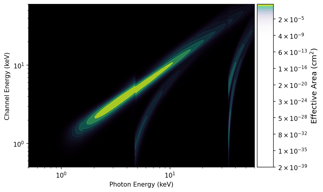
What we see in the plot is a diagonal edge that contains a majority of the effective area. This approximately linear mapping of photon energy to energy channel is called the photopeak. There is also a bunch of off-diagonal contribution from photons deposited into energy channels lower than the original photon energy. This presence of non-negligible off-diagonal response is one of the reasons that the DRM is not invertible (our lives would be so much easier if was, though).

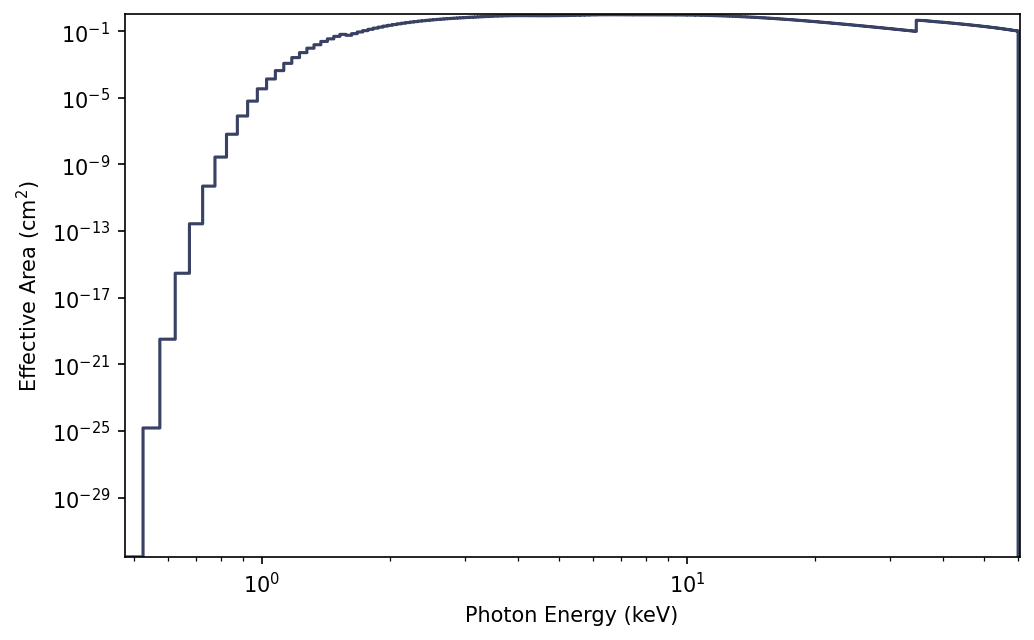
We can also make a plot of the effective area integrated over photon energies using PhotonEffectiveArea:

>>> from gdt.core.plot.drm import PhotonEffectiveArea
>>> effarea_plot = PhotonEffectiveArea(rsp.drm)
>>> plt.show()

For more details about customizing these plots, see Plotting DRMs and Effective Area.

Reference/API

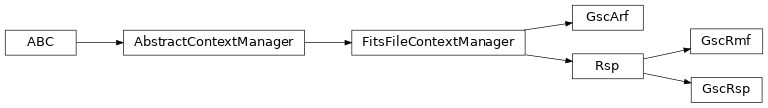
gdt.missions.maxi.gsc.response Module

Classes

GscArf()	A MAXI GSC Ancillary Response File (ARF)
GscRmf()	A MAXI GSC Response Matrix File (RMF)
GscRsp()	Class for MAXI GSC response files

Class Inheritance Diagram